Introduction
The numerical model that you can download from this page is a "moist- radiative-convective" model of the atmosphere (RMCM). It includes a simplified representation of the hydrological cycle (evaporation, condensation, cloud formation and precipitation).
This model is able to simulate the adjustment of the temperature of the atmosphere to equilibrium under influence of absorption of incoming Solar radiation and absorption and emission of terrestrial radiation and release/consumption of latent heat. You will investigate the dependence of the global average equilibrium temperature distribution as function of height on the concentration of the well mixed greenhouse gas (carbon dioxide), and the availability of water at the surface for evaporation, which depends on the Bowen ratio (ratio of sensible heat flux at the surface to latent heat flux at the surface). You will come to understand the existence of a troposphere and a stratosphere and find an answer to the question why the tropopause (the boundary between the troposphere and the stratosphere) is so "sharply" defined and is found at a height of about 10-15 km above sea level. You will investigate the water vapour feedback and the two-fold role of clouds in determining the temperature of the atmosphere. It is also possible to investigate the role of ozone.
The figure to the right shows the equilibrium temperature as a function of pressure according to the model (blue) with prescribed insolation of 341 Watts per square metre (Solar constant=1365 Watts per square metre), compared to the temperature profiles in the so-called "US 1976 standard atmosphere" (red) and in the northern hemisphere (south of 80°N) of the so called "COSPAR International Reference Atmosphere" (black). The agreement between the model and the US standard atmosphere is very satisfactory. The CIRA temperature is about 5 K lower at the tropopause. This is probably due to the biass towards the tropics which are much colder at this height than at higher latitudes.
Cloud cover fraction is prescribed at 0.6; surface evaporation is prescribed to be 80 Watts per square metre; cloud albedo is 0.45; ground albedo is 0.1; mixing ratio of "carbon dioxide" is 353 ppm, water vapour scale height is 2 km. More details can be found in the documentin chapter 2 of the lecture notes on Atmospheric dynamics. The input is specified in an input file (InputRMCM...).
Interesting model-results are the precipitable water (24.9 mm) and the sensible heat flux at the surface (13.2 W/m^2), both reasonably in agreement with observations.
Background theory
The determination of the different terms in the energy balance of the Earth-atmosphere system is a task that has occupied many researchers since the end of the 19th century. The subject is of great importance because it stands at the centre of the discussion on the greenhouse effect. With the advent of satellites the accuracy of determination of the energy fluxes (of Solar radiation and of terrestrial radiations) at the top of the atmosphere is determined with relatively great accuracy. However, there is still a great deal of uncertainty about how much of the Solar radiation is absorbed in the atmosphere, about the role of clouds in the radiation budget and about the non-radiative fluxes at the Earth's surface (the sensible heat flux and the latent heat flux). A recent paper on this subject can be downloaded here: Paper. Read this paper!
The following document contains all necessary information about the model, including a description of the method used to incorporate the water cycle and clouds.
Study chapter 2 of the lecture notes on atmospheric dynamics, in particular section 2.7, which is a description of the first most simple version of the model, which does not take account of the effects of the water cycle.
Sections 2.11-2.17 contain the description of version 15 of the model, which includes absorption of Solar radiation by ozone and water vapour, the spectral depence of absorption and emission and the water cycle (evaporation, clouds, precipitation). Solar radiation is split into 4 spectral "channnels", while and infra-red radiation is split into 3 spectral "bands". The infrared window is one of these bands. Precipitable water (PW) is a prognostic variable. PW and water vapour density at the Earth's surface determines the water vapour density profile, given its scale height (the water vapour scale height is about 2 km). Relative humidity at the ground determines cloud cover. Clouds absorb infrared radiation in all three wavelength intervals. Solar radiation is absorbed by water vapour and ozone. Precipitation is modeled as a relaxation proces towards a height dependent reference value of the relative humidity
The source code of the model
Originally the model was programmed in the programming language PASCAL. Carleen Tijm-Reijmers has now made a FORTRAN version.
The PASCALsource code of the program is contained in the following file: RMCM15.p (a text file). This is version 15 of the model (October 2012-January 2014). Download this source file and place it on the Desktop of your Apple Mac computer. The file-name must be RMCM15.p. To run this version of the program, you must also download the inputfile (InputRMCM15), as well as the file containing the observed distribution of ozone in the atmosphere , which is prescribed in the model (O3mixingratio_25x31) and CIRAandSA_25, which contains the CIRA (COSPAR International Reference Atmosphere; Fleming et al., 1990) and SA (US1976 Standard Atmosphere) temperature profiles at the 25 model levels. Likewise, the O3mixingratio_25x31 -file contains the global and annual average distribution of ozone at the 25 model levels. If you set the number of levels to a different value than 25 you will need to interpolate the ozone concentration to the appropriate grid. Download the input files and place them in the folder /Users/Shared/WorkFolderRMCM15/Input. You must also make a folder: /Users/Shared/WorkFolderRMCM15/Results.
RCM.p is the oldest version of this program, where the absorption of solar radiation by the atmosphere is neglected, the mixing ratio of greenhouse gases is constant and the hydrological cycle is not taken into account.
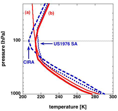
Radiative-conevective equiibrium temperature a a function of pressure in an atmosphere that is "grey" to long wave radiative transfer for two cases, compared to the "observed" COSPAR International Reference Atmosphere (CIRA) annual average temperature of the northern hemisphere (blue long-dashed curve) and the US-1976 Standard Atmosphere (SA) (blue short-dashed curve). In case (a) the "clear sky" atmosphere is transparent to Solar radiation. In case (b) ozone absorbs Solar radiation.
Exercises
Run the model with the parameter values set to the values given in the input file as downloaded. Compare the output with the observations: CIRAandSA_25. (COSPAR International Reference Atmosphere and US Standard Atmosphere).
Investigate the effects of ozone, carbon dioxide, water vapour, clouds (albedo effect and greenhouse effect), soil moisture and Bowen ratio by changing the values of the appropriate parameters and rerunning the model to equilibrium. Investigate the water vapour feedback. Compare the model energy balance with the observed global and annual average energy balance (figures 2.10 and 2.25 in the lecture notes on the energy balance). Is the cloud cover produced by the model realistic? What about the precipitable water and the precipitation rate?.
Instructions on running the program
Create a new folder in /Users/Shared/ and name it WorkFolderRMCM13. Within this folder you must create two new folders named Results and Input. The inputfile InputRMCM13 should be located in this folder. The files containing the initial temperature distribution and the prescribed ozone distribution should also be located in this folder. The name of this file is specified in the inputfile. The output of the programRMCM13.p will also be stored in the folder Results.
To compile the program on the (Apple Mac) computer you must start up X11 or Terminal. You will then enter the UNIX operating system. Now, go to the Desktop by entering the following command.
cd Desktop
The program is formulated in PASCAL. Therefore, you must invoke the Pascal compiler to compile the program. Enter the following command.
gpc RCM.p
(RCM.p is the oldest version of the program). The computer now produces an executable file from the source file *. This new file is called a.out and is also located on the Desktop. To run the program you just type the following command.
./a.out
You will find two output files in the folder /Users/Shared/WorkFolderRMCM10/Results. The first file contains the time evolution in terms of temperature (etc) and the last file containsthe energy fluxes, evaporation rate, precipitation rate, planetary albedo and cloud cover (etc). These files can be read by the program KALEIDAGRAPH (running under OS-X). With this program you can analyse the data by making graphs and scatter plots, etc.
*An executable file that will run faster can be generated with the following command.
gpc -O3 -funroll-loops -msse3 RCM.p
Compilation time is longer than with the original command (gpc RCM.p).
References
Fleming, E. L., S. Chandra, J. J. Barnett, and M. Corney, 1990: Zonal Mean Temperature, Pressure, Zonal Wind, and Geopotential Height as Functions of Latitude. Advances in Space Research, 10, No. 12: CIRA.