I appreciate it very much you are taking your time to attend the virtual version of EGU. These are strange times, and I can imagine it feels like your work is presented somewhere in the void. However, this also brings an opportunity, especially to change the way we communicate our science. Thus even though we can not meet in person, I have tried to make this presentation an experience. Thus please scroll through, and if reading is not your thing, enjoy my work through my vocals!
Copyright: All rights are reserved, but I still grant Copernicus Meetings the right to hold my presentation materials online for viewing and download by individuals. Background starting and closing image are from imagegeo.
Rationale
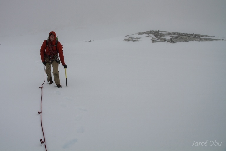
My research is mostly concentrated around glacier velocity or elevation change, at different time scales. In the last years, I have worked on automatic extraction of surface displacements from optical remote sensing. It is amazing we are able to generate such time-series of velocity evolution from space and learn from these products. Now that we have the tools, more phenomena can be seen, but lets first start with how I came to conduct this study.
If we think about glacier debris, many people have a first association with erosion, but I see it as markers of glacier dynamics. For example the position of a medial moraine band is a relation between the relative ice throughput of two glaciers. When the location of a moraine band is stable over time, it seems to resemble a streamline, or stated differently, it describes the trajectory a particle had or will flow through the glacier. But a change in glacier flow can result in an alteration of location for this moraine band, in this case it is more clear that supra-glacial debris functions as a streakline. What I mean with this, can for example be seen in the simulation of debris on a glacier in the video.
Thus when I see looped, curved, or wiggly moraines, I instantly think about flow instability and how these glacier systems have interacted. It is from this perspective, I look at debris covered glaciers. However, their flow velocity is in general very low, but there are more flow markers present on a glacier! Typically, emerging or deposited debris functions as an isolating blanket for the glacier ice underneath. While the opposite can also occur when energy from the heated debris can be transferred to the ice, either because the layer is thin or not homogeneous. Differential melt due to these different debris distributions cause changes in local topography. Over time larger topographic gradients emerge, causing debris to move in local down-slope direction. This is a feedback mechanism, that occurs on many debris covered glaciers, and in its extreme form, these result in ice cliffs, with almost vertical walls and blank ice. An ice-cliff face melts away in a direction perpendicular to its normal surface, thus instead of down-wasting, it will propagate horizontally as well. Thus over time the crest or top of the ice cliff moves in opposite direction of its own aspect. But these ice cliffs are occurring on the surface of a glacier, so are super imposed on the glacier flow. Hence, when we want to track ice cliffs, two signals need to be sensed, one of general glacier flow, and one of individual ice cliff migration. This can become a mess, as can be seen in the animation which shows a simulation of these combined processes.
Debris is in black and flows along with the ice, the glacier is symmetric and maximum in the middle. Ice cliffs are in gray, and have a dominant orientation towards the South, as there seems to be a preference for this orientation.
In this work in want to disentangle these two movement patterns. The whole thing is sprung from an opportunity, but I think it can also contribute to a better understanding of the evolution of debris covered glaciers. If the movement over time can be tracked over several glaciers, it might become possible to do regional assessments, and learn from differences and relating factors. While ice cliffs occupy only a small area of the glacier surface, they are a significant contributor to glacier melt in the lower parts of a glacier. Elevation-dependent melt models only weakly capture the ablation patterns of debris covered glaciers, as debris covered snouts seem to down-waste over their entire debris covered surface on decadal time-spans. On shorter time scales, it seems these swiping ice cliffs over are an important process, so quantitative numbers for such phenomena is of interest.
An extensive amount of research has already been done on these ablation features, but these have mostly been focused on small scale processes or individual ice cliffs. We hope with this work, we can contribute to this understanding by giving tools to up-scale to more ice cliffs.
Venus
In our study we use data from the venµs satellite, this data is provided freely through the THEIA portal
The venµs satellite is an optical satellite missions, that demonstrates the opportunities of high repeat space borne remote sensing. It acquires imagery over 100 sites, of which a handful are situated in mountainous or arctic regions. The instrument senses with twelve spectral bands in the visible spectrum, with a resolution of 5 meters and a swath width of 27.5 kilometers. Currently, the archive consist of three years of data, but it is ending this part of the mission. However, it is sufficient enough time for this study and show the potential for monitoring of glaciers with debris cover.
Khumbu Glacier
The region we use as a test case is Khumbu Glacier and its surrounding, which covers Mount Everest and many other debris covered glaciers. On the southern flank of Mount Everest snow accumulates in the Western Chm glacier, which flows through an icefall into Khumbu Glacier (at rates of 500 meters per year). The equilibrium line altitude (ELA) is in the icefall of clean ice, but not long after the icefall debris starts to emerge. Also the flow slows down and is in the order of 100 meters per year, and at the confluence with Changri Shar Glacier has slowed down significantly. Ice flow lower down the debris covered tongue are in the order of 10 meters per year or less. Using images from venµs that are taken one year apart from each other, it is possible to see changes on the surface. For example below you can see both movement of ice cliffs, as well as ice. This is the starting point and the data to work with!
On the left here is a gray bar, which is a slider, so you can look at the difference between 2019 & 2020. It works in Chrome and Firefox, but not in Edge.
methodology
The idea behind this work, is that two processes are occurring, but this results in transmitting different signals which eventually compose an image. The ice cliffs are topographic features, and are thus an illumination signal (shadows and shading). While debris on a glacier can have a distinct reflectivity signal (rocks have fifty shades of grey). Furthermore, the spatial scale of velocity is different; backwasting of ice cliffs is local, while glacier ice flow is slowly varying.
Thus if we can separate the illumination from the reflectivity, we can concentrate on the ice cliffs or the lithology. Because the venµs satellite has a multi-spectral instrument, sensing each location multiple times, there is redundancy which makes separation possible. For example, the image below shows a false color image of a section of Khumbu and Changri Shar Glacier, and the estimated illumination component of this image.
On the left here is a gray bar, which is a slider, so you can look at the difference between a false color image and the estimated illumination image
With the estimated illumination image we are able to enhance shading features and shadowing features. If we concentrate ourselves to the shadows and think of an ice cliff in the shade, the shadow edge we see with the satellite is of a particular shape and is composed of two regions. The region closest to the sun, blocks illumination for the locations further away from the sun. While the other shadow edge region is at the outer-end and is the transition zone where direct illumination by the sun is possible again. Thus the former is in the self-shadow region, while the later is in the cast-shadow region. Another way of looking at this is from the illumination angle in respect to the shadow edge orientation. Locations of a shadow edge, which are also in self-shadow, have an orientation or aspect that never surpasses a right angle from the illumination direction. While cast shadow edges, occupy the other half of orientation angles. This feature is of importance, as we are interested in the crest of ice cliffs, which are the shadow edges in the self-shadowing domain. These location can thus simple be extracted from their orientation.
We will thus be using these ridges of ice cliffs and follow their movement over time. However, in order to validate our metholodology we need to be able to assess if our estimates are legitimate. Therefore another feature of the venµs satellite needs to be explained first.
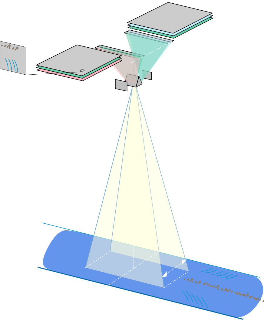
The venµs satellite has an instrument onboard with several multi-spectral line-arrays. These are lined-up next to each other, and perpendicular to the flight direction of the satellite. As the satellite flies its orbit, the different sensor arrays acquire data in a pushbroom fashion. The recording at every time instance, results in a row within a satellite image. However, the multi-spectral recording are not instantaneous, as a small time delay is present for acquisitions of a certain location (up to 2.7 seconds). Furthermore, the look angles of every photo array is a little bit different. Consequently, a small parallax angle is present (of almost three degrees). This is a general feature for any multi-spectral pushbroom satellite and thus also true for the venµs satellite. This effect is especially clear because of the large collection of multi-spectral arrays within the instrument. In order to minimize this effect within the satellite instrument, a system of prisms is used to diffract the light coming into the telescope. One design feature of venµs, we exploit in this study, are two line arrays that are both at opposing ends of the sensor, but that have the same spectral sensitivity. Here pixel shifts are directly related to orthorectification errors. Its intended purpose is to detect clouds, but it is also possible to see high resolution deviations, like ice cliffs!
Using these nice features of the venµs satellite, we are able to generate a geometric signal of ice cliff migration as well! For a single image, we can get cliff crests, and geometric undulations, as is shown below. As you might see, a similar pattern is observable, though they stem from two completely different principles.
On the left here is a gray bar, which is a slider, so you can look at the difference between detection of ice cliffs through the illumination method, or though photogrammetry
The last step in the methodology is to isolate the different ice cliffs and track their movement over time. The time span of the imagery is exactly one year, so the illumination direction is constant. However, this might not be a hard prerequisite, as sun synchronous satellites have a fixed local overpass time. Matching of the ice cliffs gives than the combined migration and iceflow, while matching of the reflectivity image gives the general glacier flow.
Results
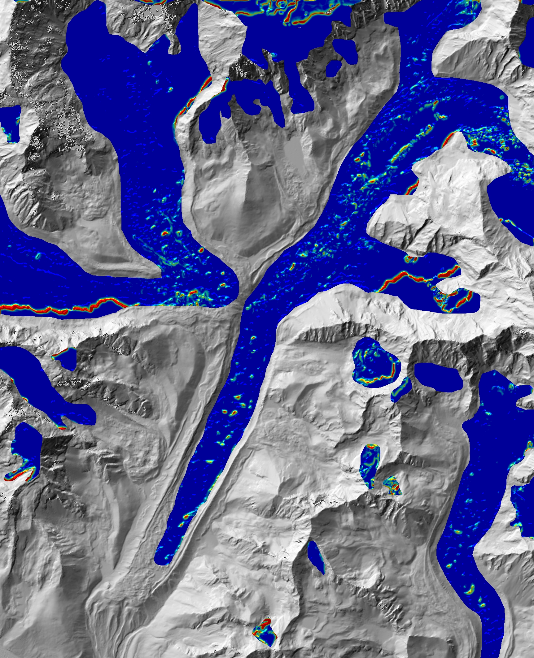
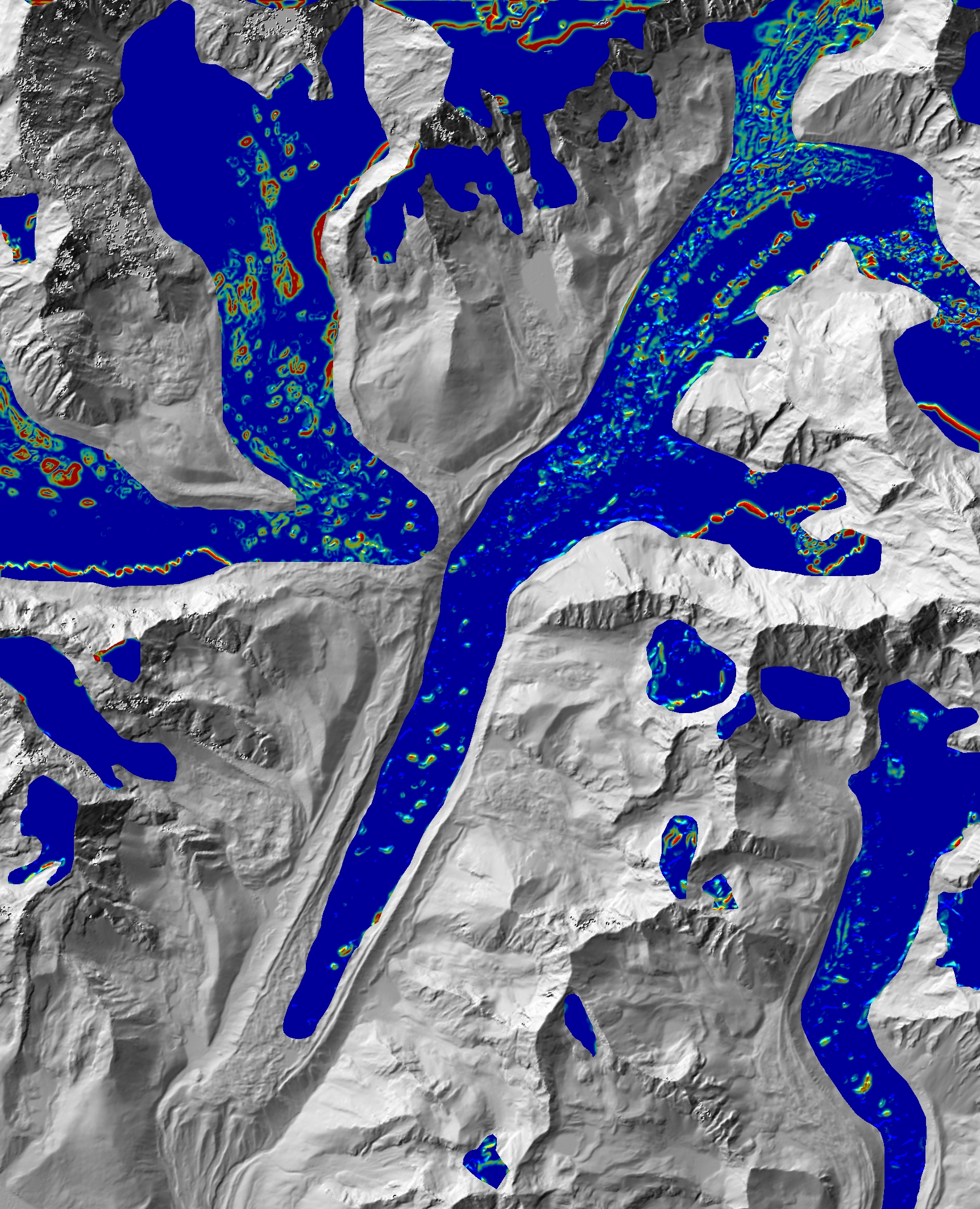
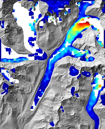
The identification of the ice cliffs is done through detecting of the self-shadow edge and these are highlighted in the figures below (they have bright colours). This mask is draped over the color coded ice-cliff movement estimation, so you can get a clear idea of the localization of ice cliffs and the movements we extract (which are the colors). There is no filtering applied, so also cast shadows of crevasses or mountains are here included in the results. The movement of ice cliffs seems to be estimated correctly.
ice cliff speed in 2018
ice cliff speed in 2019
You can move your cursor over the image (on the right), to see a zoomed version (on the left).
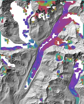
general glacier flow
The results are split up in magnitude and orientation, to give a better "feeling" about the surface velocities. For these results the general flow estimation is done through the reflectivity component of the imagery and seems to give the general glacier surface flow pattern. However, the reflectivity component at some regions in the imagery are of low variability (snow). At these places the matching is not reliable and left out here. Other regions have fast flow (the icefall) and matching is complicated as well, hence are also left out. Overall, the general flow is captured and it seems it is possible to separate the general ice flow from the local ice cliff movement!
magnitude
orientation
This is still work in progress, and some elements might be possible to optimize or improve. Furthermore, up-scaling towards the whole Everest region is not yet done, but since everything is automatically generated, not much hurdles are foreseen. Another outlook is to test if this methodology is transferable to Sentinel-2: this will be more challenging, as its pixel resolution is ten meters, but this will make large scale assessments possible. We are anyways very happy, as it seems to be possible to extract such type of backwasting information, and we hope it can be of use for the community!
Thank you, for taking your time!
feel free to contact us! or connect through twitter: @baasaltena
Institute for Marine and Atmospheric research Utrecht (IMAU)
Utrecht University
the Netherlands
Department of Geosciences
University of Oslo
Norway